Summarize Campaign Data

Introduction

You’ve received some campaign results that contain one row for each source code and you want to summarize this data. This is the perfect use case for a Pivot Table. In this guide, we’ll take some sample campaign data at the soruce code level and transform it into an interactive, summarized campaign report.

The data we will be working with looks like this:

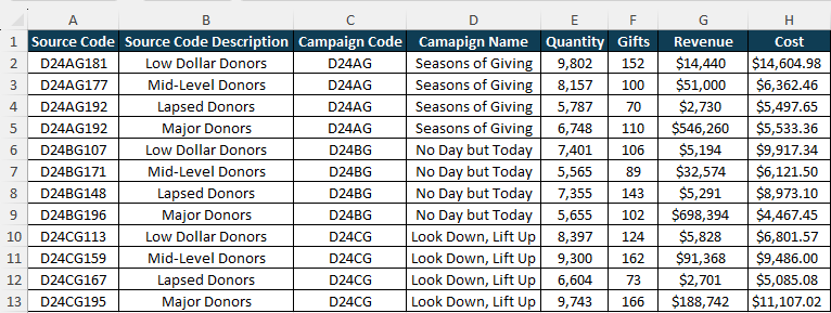
We will summarize the data in a pivot table, allowing us to:

• Create calculated fields like response rate and average gift
• Group results by campaign
• Drill into campaign-level results to see segment-level performance
• Filter for specific campaigns or segments

1. Create a pivot table

Pivot tables are powerful tools that help you quickly summarize and analyze large sets of data without needing complex formulas. Think of them as dynamic reports that let you easily group, sort, and filter your data. With just a few clicks, you can rearrange your data (extremely Ross Geller voice: pivot it) to view insights from different angles.

Creating a pivot table from source data that’s already in Excel is quick and easy. Just select the data you want to include in your pivot table and then select Insert > PivotTable from the ribbon and click “ok” on the resulting dialog box:

2. Pivot your data

Pivot tables can be populated with a simple drag-and-drop system. When you created your pivot table, a section of options labeled “PivotTable Fields” opened up on the right side of your Excel window. There are five parts to this section, each described below:

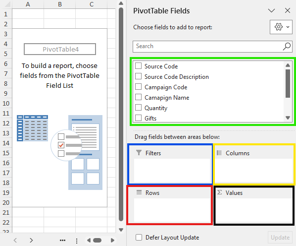
• Field Listing (green box): this area lists every column from your original data. You can click and drag these columns into the four boxes below to pivot your data.
• Filters (blue box): dragging a field into this box makes that field available as a filter on your report
• Columns (yellow box): dragging a field into this box puts the values from that field into the columns of your report
• Rows (red box): dragging a field into this box puts the values from that field into the rows of your report
• Values (black box): dragging a field into this box puts the values from that column into the main area of the report, this is where you’d include a numeric field like “Revenue” or “Gifts”

It’s easier to see how this all works with an example. We’ll manipulate our pivot table to summarize total revenue by Source Code Description. To do this, we will drag the “Source Code Description” field from the field list into the Rows (red box) and drag the “Revenue” field into the Values (black box):

So what just happened? Excel did a couple things for us:

• Each unique value for Source Code Description (across all of our campaigns) turned up as a row in our report
• The sum of all the revenue from those Source Code Descriptions (across all of our campaigns) was displayed next to their respective descriptions

With a couple clicks, we’ve got revenue by Source Code Description.

3. Pivot by campaign name

We also want to know how much of the revenue from each of these Source Code Descriptions came from each of our campaigns. To do this, we can drag the “Campaign Name” field from our field listing into the Columns area (yellow box):

This cross-tabluates the revenue by Source Code Description and Campaign Name so that we can see total revenue for each description, for each campaign, along with totals for each independently as well as a grand total for all the revenue.

4. Create a calculated field

Finally, we want to add response rate to our report using a calculated field. To create a calculated field, head up to the ribbon and select Pivot Table Analyze > Fields, Items, & Sets > Calculated Field. You’ll get a dialog box asking for the Name of your new field and the Formula to calculate.

You can name the field anything you’d like, we’re going to go with “Response Rate” in our example. The formula works like any other Excel formula, it starts with an equals sign and is a mathematical expression. We’re going to enter =Gifts/Quantity to calculate response rate, then click “OK”:

Ok what happened here? Why is Response Rate showing 0 for everything? This is happening becasue Excel doesn’t know that Response Rate is a percentage, it thinks it’s just a number, so a value like 0.015 is being rounded down to 0 rather than displayed as 1.5%. We’ll fix this and use some more pivot table functionality to make the report easier to read.

5. Formatting your report

Let’s reformat our report so that it’s eaiser to read from top to bottom and so that our Response Rate shows up as a percentage.

Format the response rate

To format the response rate, right-click anywhere you see “sum of Response Rate” and select “Value field settings…”. In the dialog box, click the “Number Format” button in the lower left corner, select the “Percentage” category, and choose 2 decimal places. Then click OK:

There, now our response rates are nice and pretty. But the report is still kind of hard to read.

Reorganize the table

We’ll make it so that each Source Code Description is nested within each campaign, allowing the report to be read from top to bottom more easily. To do this, drag the “Campaign Name” field from the “Columns” box to the “Rows” box, and put it on top of Source Code Description. This will even allow us to collapse the Campaign Names to allow users to drill down into the Source Code Descriptions:

6. Keep working

We’ve barely scratched the surface of what pivot tables can do and how you can use them to build campaign reports. In the sample Excel file for this guide, I’ve built out the example you see in these short videos along with several other examples with some additional hints and tips. Learning to create reports like this using pivot tables takes a bit of time playing around with what’s possible, but with a small amount of practice, you’ll be an expert in no time.